Deploying a Time Series Foundation Model on SageMaker for Zero-Shot Forecasting
- 10 minsMost teams build one model per time series. This post is about deploying a single foundation model that forecasts any time series without training. Google's TimesFM 2.5—a 200M parameter decoder-only transformer pre-trained on 100 billion real-world time points—goes from raw numbers to calibrated probabilistic forecasts in a single forward pass. No feature engineering, no per-series tuning, no training pipeline.
The inspiration comes from the same shift we saw in NLP: instead of training a new classifier for every task, you pre-train once on massive data and deploy zero-shot. TimesFM does this for time series. The core loop doesn't change: patch the input, attend to prior context, project the next output patch. Everything else—SageMaker, ECR, async inference, auto-scaling—is the infrastructure to make that loop accessible as an API that costs $0 when idle.
From raw cost history to calibrated forecasts and anomaly detection in one API call.
The model
TimesFM 2.5 with 200M parameters. 20 transformer layers, 1280 model dimension, 16 attention heads with RoPE positional encoding, SwiGLU activations, and RMSNorm. Input patch length of 32, output patch length of 128. Context limit of 16,384 time points. Only the architecture is custom—everything else is a standard causal decoder, the same family as GPT and Llama. “Predict the next patch” instead of “predict the next token.”
The asymmetric patching is the key insight: input patches are 32 points, but output patches are 128. This means each autoregressive decode step forecasts 4x more than it consumes. A 256-point forecast needs only 2 generation steps instead of 8. Less error accumulation, faster inference.
Pre-trained on 100 billion time points from Google Trends, Wikipedia pageviews, and public time series datasets. The model learns temporal patterns—trends, seasonality, noise—without knowing what the data means. It doesn't know “Monday” or “holiday” or “Black Friday.” It just knows shapes.
The output: point forecasts plus 9 quantiles (10th through 90th percentile) giving calibrated prediction intervals. You get uncertainty for free.
The setup
The goal: deploy TimesFM as an API endpoint that accepts arbitrary time series, returns forecasts with uncertainty bands, and costs nothing when nobody's using it.
Hardware: 1x ml.g5.xlarge on SageMaker—a single NVIDIA A10G with 24 GB VRAM. The model uses about 2 GB. The rest is headroom for batching hundreds of series simultaneously.
Container: AWS PyTorch Deep Learning Container (PyTorch 2.6, Python 3.12, CUDA 12.4) with transformers>=5.3.0 installed on top. The TimesFm2_5ModelForPrediction class handles everything: loading weights from HuggingFace Hub, patching, attention, decoding.
Inference pattern: SageMaker Async Inference with auto-scaling to zero. Requests go to an internal queue. If no instance is running, auto-scaling spins one up (~3-5 minutes cold start). After 10 minutes idle, it scales back to zero. You pay $1.20/hr only when actively running forecasts.
Infrastructure: Terraform. One terraform apply creates the full stack—IAM role, ECR repo, S3 buckets, SageMaker model, endpoint configuration, endpoint, auto-scaling policy.
Infrastructure
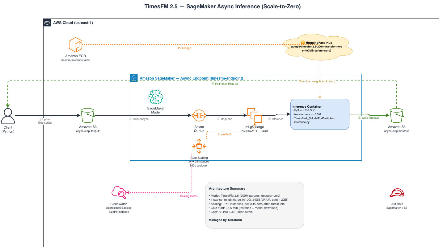
The infrastructure is two layers: Serving (SageMaker endpoint with the custom container, async queue, auto-scaling from 0 to 2 instances based on queue depth) and Storage (S3 bucket for async input/output, ECR repository for the container image).
The Terraform creates: ecr_repository, iam_role, s3_bucket, sagemaker_model, endpoint_configuration, endpoint, appautoscaling_target, and appautoscaling_policy. Everything is parameterized:
variable "instance_type" {
  default = "ml.g5.xlarge"
}

variable "scale_to_zero_idle_seconds" {
  default = 600
}

variable "max_instance_count" {
  default = 2
}
The container image is minimal—a Dockerfile that installs transformers on top of the DLC base:
FROM 763104351884.dkr.ecr.us-east-1.amazonaws.com/pytorch-inference:2.6.0-gpu-py312-cu124-ubuntu22.04-sagemaker

RUN pip install --no-cache-dir \
    "transformers>=5.3.0,<6.0" \
    huggingface-hub safetensors

COPY inference.py /opt/ml/code/inference.py
ENV SAGEMAKER_PROGRAM=inference.py
The inference.py defines four functions that SageMaker's serving toolkit calls: model_fn loads the model from HuggingFace Hub at container startup, input_fn deserializes JSON, predict_fn runs the forward pass, output_fn serializes the result. The entire inference handler is 50 lines:
def model_fn(model_dir):
    model = TimesFm2_5ModelForPrediction.from_pretrained(
        "google/timesfm-2.5-200m-transformers"
    )
    model = model.to(torch.float32).eval()
    if torch.cuda.is_available():
        model = model.to("cuda")
    return model

def predict_fn(data, model):
    past_values = [torch.tensor(ts, dtype=torch.float32) for ts in data["inputs"]]
    device = next(model.parameters()).device
    past_values = [pv.to(device) for pv in past_values]

    with torch.no_grad():
        outputs = model(past_values=past_values, forecast_context_len=1024)

    return {
        "point_forecast": outputs.mean_predictions[:, :horizon].cpu().numpy().tolist(),
        "quantile_forecast": outputs.full_predictions[:, :horizon].cpu().numpy().tolist(),
    }
Deployment is three commands:
cd container && ./build_and_push.sh    # Build image, push to ECR
cd terraform && terraform init
terraform apply                         # ~5 minutes for the full stack
Teardown: “terraform destroy tears down the endpoint. ECR repo is protected (no re-pushing 10 GB). No ongoing costs.”
Results
Results below reflect forecasting on 366 days of daily AWS cost data across 10 services, using the deployed SageMaker endpoint.
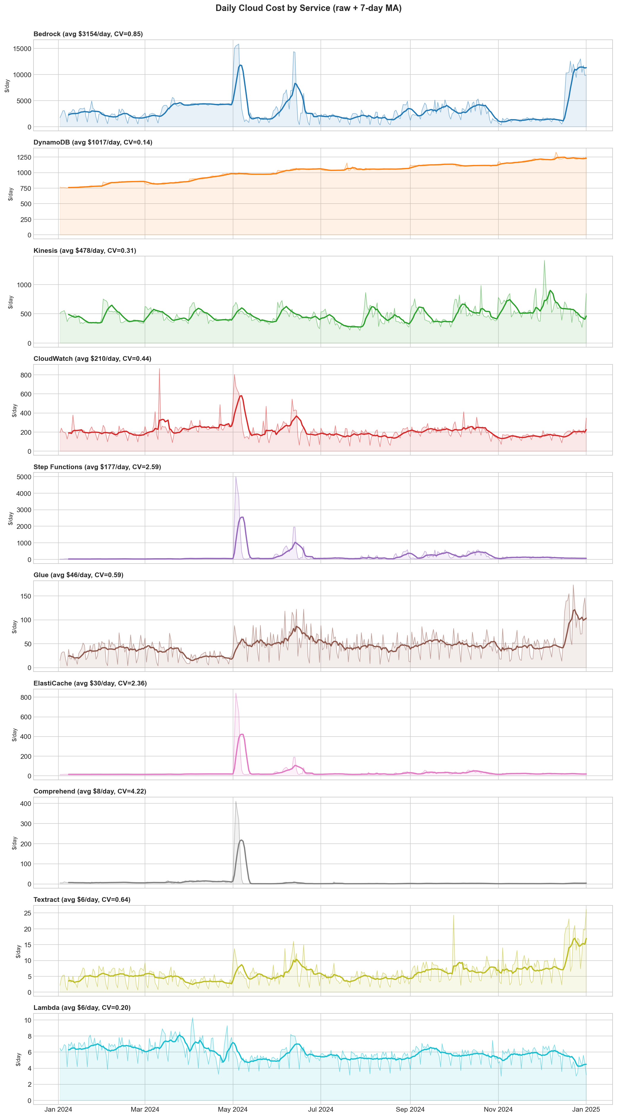
The dataset: daily AWS costs from January 2024 through January 2025. Ten services ranging from $6/day (Lambda) to $3,154/day (Bedrock). Coefficient of variation from 0.14 (DynamoDB, steady) to 4.22 (Comprehend, extremely bursty). This is not toy data—it has regime changes, spikes, seasonality, and flat periods.
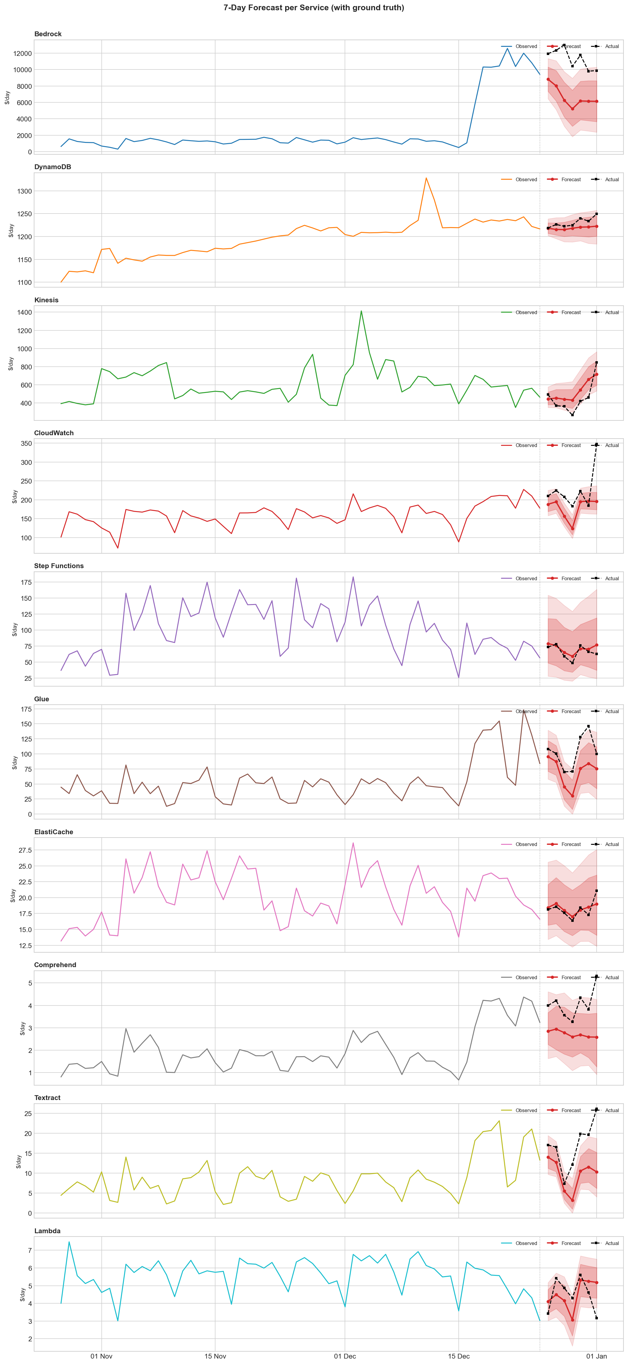
Three forecast horizons tested per service: 7-day (short-term, validated against held-out ground truth), 30-day (monthly budget planning, validated), and 90-day (quarterly projection, no ground truth).
7-Day forecast accuracy:
| Service | Avg $/day | MAE | MAPE |
|---|---|---|---|
| DynamoDB | $1,017 | $12.03 | 1.0% |
| ElastiCache | $30 | $0.78 | 4.2% |
| Step Functions | $177 | $6.67 | 10.9% |
| CloudWatch | $210 | $50.47 | 20.4% |
| Kinesis | $478 | $119.47 | 29.3% |
| Bedrock | $3,154 | $4,619.32 | 40.8% |
The pattern is clear: stable services get excellent forecasts, volatile services get poor ones. DynamoDB storage costs grow steadily—easy. Bedrock had a regime change from $1,500/day to $12,000/day in the final week—impossible to predict from history alone.
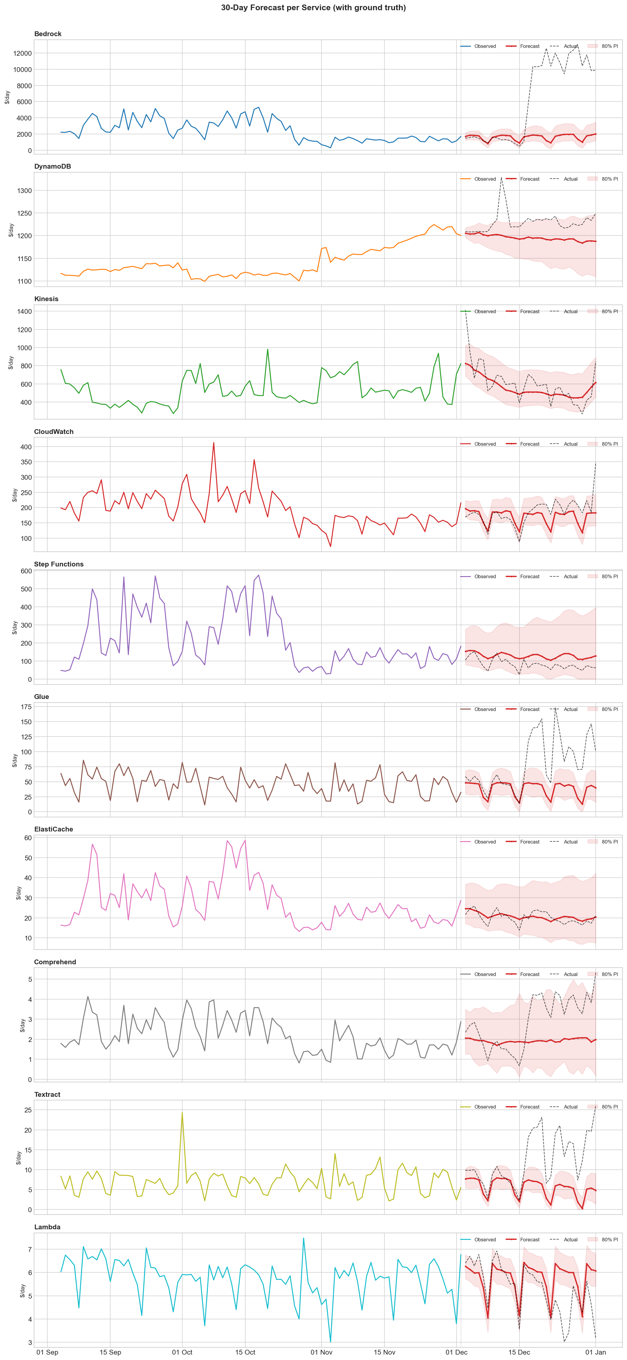
30-Day cumulative accuracy:
| Service | Predicted | Actual | Error |
|---|---|---|---|
| DynamoDB | $35,860 | $36,916 | -2.9% |
| ElastiCache | $619 | $603 | +2.6% |
| Lambda | $173 | $158 | +9.2% |
| Kinesis | $16,742 | $18,239 | -8.2% |
| Bedrock | $48,618 | $188,795 | -74.2% |
For budget planning, the cumulative errors matter more than daily errors. DynamoDB, ElastiCache, and Lambda are all within 10%—good enough for capacity planning and cost alerts. Bedrock's -74% error is the regime change: the model predicted continuation of the old baseline.
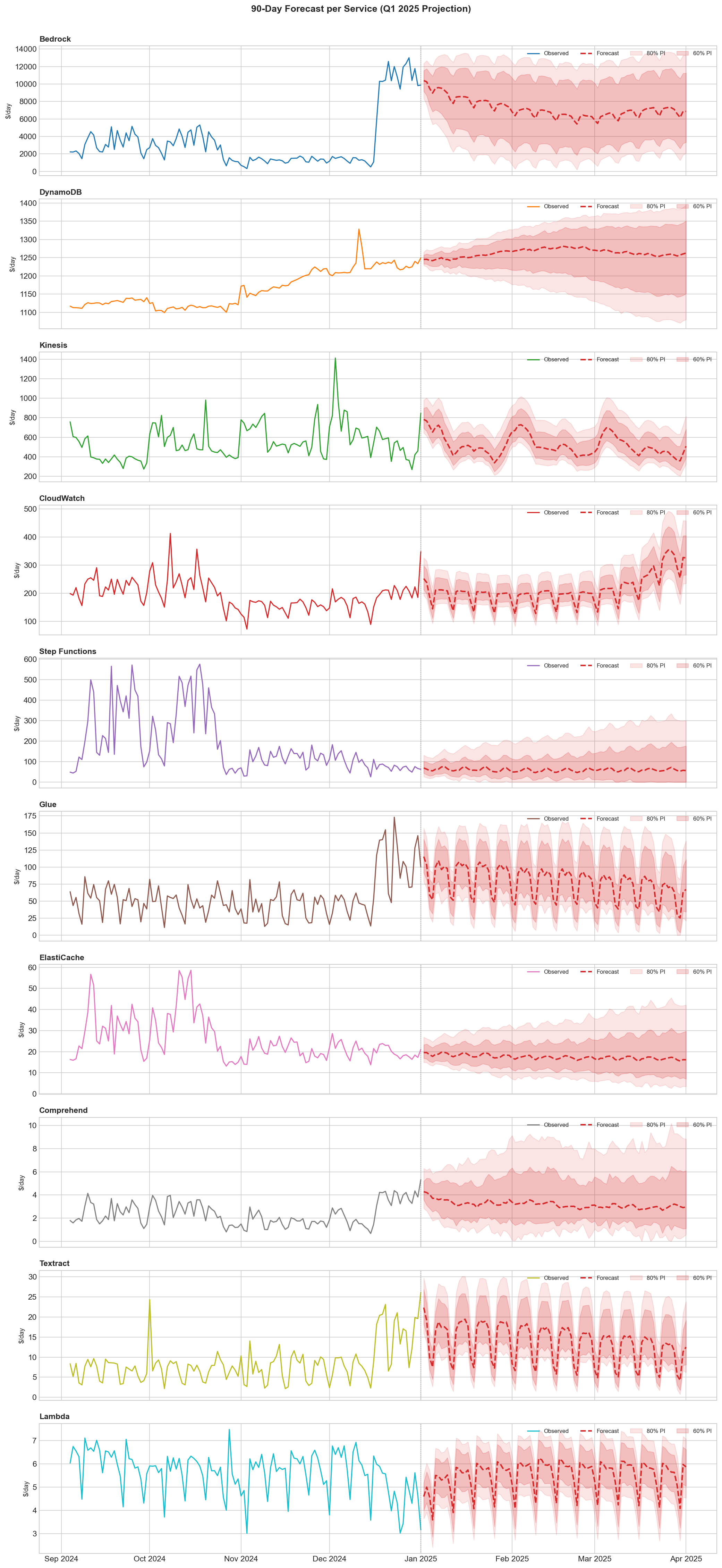
90-Day projections show appropriately widening uncertainty bands. The model is honest about what it doesn't know: Bedrock's 80% confidence interval spans $176K to $1.15M. For DynamoDB: $103K to $121K—narrow, because DynamoDB costs are predictable.
Anomaly detection
The same model that forecasts also detects anomalies. The approach: run rolling 7-day forecasts using only past data, then flag any day where the actual cost falls outside the prediction intervals.
- CRITICAL: actual cost outside the 80% PI (q10–q90)
- WARNING: actual cost outside the 60% PI (q20–q80)
A minimum threshold of $5 or 20% deviation filters out noise on tiny fluctuations.
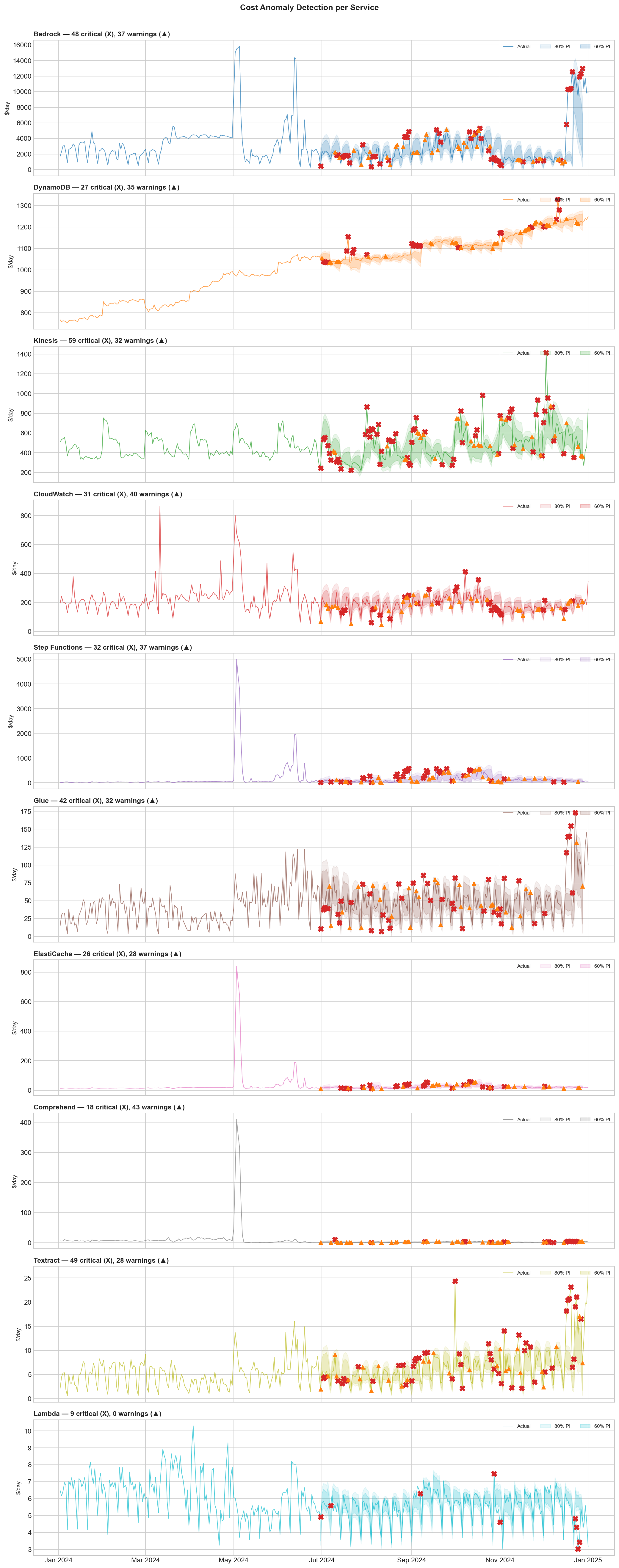
Top anomalies detected:
| Service | Date | Actual | Expected | Delta |
|---|---|---|---|---|
| Bedrock | 2024-12-21 | $12,580 | $827 | +$11,753 |
| Bedrock | 2024-12-28 | $13,003 | $4,121 | +$8,882 |
| Kinesis | 2024-12-03 | $1,414 | $650 | +$763 |
| Step Functions | 2024-08-30 | $587 | $81 | +$507 |
| CloudWatch | 2024-10-08 | $413 | $239 | +$174 |
This is the model's real value in production: not predicting the future perfectly, but telling you when the present is abnormal. The Bedrock spike in December—clearly a new workload deployment or scaling event—would have triggered an alert on day one. No anomaly labels needed, no threshold tuning, just “this doesn't look like what came before.”
What I learned
Zero-shot works for steady-state, fails on regime changes. If your Bedrock spend has been $1,500/day for 300 days, the model will predict $1,500/day tomorrow. If it suddenly jumps to $12,000, the model is useless for that first day—but it immediately detects it as anomalous. The forecast catches up within a few days of new context.
Async inference with scale-to-zero is the right pattern for sporadic workloads. You don't need a GPU burning $1.20/hr 24/7 for a forecast that runs once a day. The 3-5 minute cold start is acceptable for batch forecasting jobs. If you need sub-second latency, keep one instance warm.
The model is a tool, not an oracle. It tells you “based on the pattern so far, here's what's likely.” When the world changes, it lags. Pair forecasts with anomaly detection (which we get for free from the same quantile outputs) and you cover both cases: accurate forecasts when things are normal, immediate alerts when they're not.
FAQ
Why TimesFM instead of Prophet/ARIMA/custom models? Prophet needs per-series fitting (minutes per series × thousands of series = hours). ARIMA needs stationarity testing and parameter selection. TimesFM takes a list of numbers and returns forecasts in seconds for all of them at once. “The gap between zero-shot and fully supervised is narrow enough that the engineering simplicity wins.”
Why SageMaker Async instead of Real-Time or Batch Transform? Real-Time keeps the instance running (expensive for sporadic use). Batch Transform spins up, processes, tears down—good for scheduled jobs but no persistent endpoint. Async gives you a permanent endpoint URL that scales to zero. Best of both worlds for bursty, unpredictable workloads.
Why the transformers variant instead of native timesfm? Simpler deployment: no custom package install, no git clone, just pip install transformers. Trade-off: you lose covariates (XReg), flip invariance, and the continuous quantile head. For pure “numbers in, forecasts out” serving, the transformers variant is sufficient.
What about multivariate? TimesFM is univariate—each series is independent. If you need cross-series relationships (e.g., “Bedrock costs drive CloudWatch costs”), you'd add a covariate model on top. The native timesfm package supports this via XReg (linear model on residuals).
How much does this cost? Idle: $0. Active: $1.20/hr per ml.g5.xlarge. A daily batch job forecasting 1,000 series takes ~30 seconds of GPU time. That's $0.01/day. The cold start (3-5 min) dominates—so batch your requests.
Can I use this for non-cost data? Yes. Any numeric time series: API latency, user signups, temperature readings, stock volumes, sensor data, inventory levels. The model doesn't know what the numbers mean. It just knows patterns.

Tareq Haschemi
just some experiments with data